Christopher Prohm

From my time to time I find myself in the situation of having to linearize graphs. Typically this issue comes up in the context of task scheduling. When tasks have dependencies among themselves, they form a directed acyclical graph. Finding an order of the tasks that respects their dependencies is called a topological sorting or linearization. In the following, I will use the term linearization, as it seems more self-explanatory. In this post I would like to discuss a simple algorithm for graph linearization and compare how this problem is solved in the context of multiple inheritance in Python.

As an example consider a simple data science workflow "prepare data", "create predictions", and "create report". A linearization of this graph is an order of the individual steps, such that all their dependencies are executed before each step itself. For this example the graph itself is already linear and can be executed as-is.

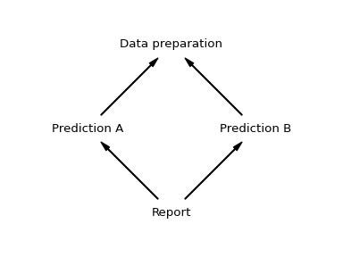
Things get a bit more complicated, if the graph contains branches. For example, if there are multiple predictions that can be executed independently, say "Prediction A" and "Prediction B". They both required the data preparation step, but otherwise can be executed in any order. Once both predictions have been created, the report task be executed.

To linearize this graph we can use a simple algorithm:

1. Traverse the graph in depth first manner and add all encountered nodes to a list, keeping any duplicates
2. Walk the list back to front and keep each item only the first time it is encountered

A Python implementation can be found at the end of the post. Note, this algorithm is effectively a less efficient variant of the the depth-first search algorithm on wikipedia. In the example, it works as follows:

# Step 1: collect all nodes in a depth first manner
["report"]
["report", "prediction-a"]
["report", "prediction-a", "data"]
["report", "prediction-a", "data", "prediction-b"]
["report", "prediction-a", "data", "prediction-b", "data"]

# Step 2: only kep each item once 
["report", "prediction-a", "prediction-b", "data]

Our example graph permits two linearizations, since the two predictions can be executed in any order, as long as the data preparation step has been executed before. Both choices are equally valid. The selected order depends on how the depth-first traversal observes the dependencies.

This simple algorithm also generalize to more complex scenarios in which the dependencies have multiple dependencies themselves.

In this example the list would be generated as

# After step 1
['A', 'B1', 'C1', 'D', 'C2', 'D', 'B2', 'C1', 'D', 'C2', 'D']

# After step 2
['A', 'B1', 'B2', 'C1', 'C2', 'D']

In the object model of Python we encounter a similar issue. Python defines a linearization of a class hierarchy, called the method resolution order or MRO. Most users interact with the MRO via the super() mechanism, which gives access to the next class in the MRO, but Python also exposes the MRO directly via the __mro__ property defined on classes. For example, the Python equivalent of the last example would be:

class LeafA(object):
    pass

class LeafB(object):
    pass

class ChildA(LeafA, LeafB):
    pass

class ChildB(LeafA, LeafB):
    pass

class Parent(ChildA, ChildB):
    pass

print([cls.__name__ for cls in Parent.__mro__])

The last line prints ['Parent', 'ChildA', 'ChildB', 'LeafA', 'LeafB', 'object']. So what algorithm is Python using to define the MRO? As it turns out Python was using the simple algorithm introduced above until version 2.2, but subsequent versions switched to the C3 linearization algorithm. Why?

While the simple algorithm is sufficient for task execution, it can lead to counterintuitive behavior for multiple inheritance. Consider an inheritance graph very similar to the one above, but with the parents of class ChildB reordered.

# NOTE: this code will note execute with python>=2.3
class LeafA:
    pass

class LeafB:
    pass

class ChildA(LeafA, LeafB):
    pass

class ChildB(LeafB, LeafA):
    pass

class Parent(ChildA, ChildB):
    pass

print([cls.__name__ for cls in Parent.__mro__])
print([cls.__name__ for cls in ChildA.__mro__])
print([cls.__name__ for cls in ChildB.__mro__])

Python versions >=2.3 will reject this code with the error "TypeError: Cannot create a consistent method resolution". The inconsistency can be observed when executing the code with older Python versions. In that case the order of "LeafA" and "LeafB" would switch depending on whether the root node is "ChildB", "ChildA", or "Parent". A graph with the property that the order of the dependencies does not change depending on the starting node is called monotonic. The C3 algorithm is specifically designed to enforce monotonicity. For any monotonic graph, it will give the same result as the simple algorithm. For any non monotonic graph, it will simply fail.

To sum up: the C3 algorithm is too strict for task scheduling. The monotonicity constraint is too strict in practice and would reject many non-monotonic task graphs that are perfectly valid in the context of task scheduling. However, it does helps to reject inconsistent class hierarchies early in the context of multiple inheritance. If you have feedback or comments, feel free to reach out to me on twitter @c_prohm.

Example implementation

from typing import Mapping, List, Sequence

def linearize(root: str, graph: Mapping[str, Sequence[str]]) -> List[str]:
    """Linearize a graph given as map ``{node: [dependencies]}``.
    """
    order = recurse(root, graph)
    order = prune(order)
    return order

def recurse(node, graph):
    yield node
    for dep in graph[node]:
        yield from recurse(dep, graph)

def prune(items):
    seen = set()
    result = list()

    for item in reversed(list(items)):
        if item in seen:
            continue

        result.append(item)
        seen.add(item) 
    
    return result[::-1]