Motivated by the recent release of Judea Pearl's Book of Why, I started to sort my notes on causality and write some parts down in a more structured way. In doing so, I stumbled over a question I bumped into repeatedly in past projects: The simplest causal system is one in which features determine actions and the combination of features and actions determine the outcome. One popular approach for this system is to apply inverse probability of treatment weighting. My intuition always was that this step should not be necessary. After some research, the answer is a resounding "Yes, but ...".
In short: no causal treatment is necessary for this system according to theory. However, causal treatment becomes important when applying function approximations with limited capacity (or AI).
The options sketched above are often discussed under the names "direct method" (no reweighting) and "inverse propensity score method" (reweighting). Both methods can be used to estimate causal effects, but typically the latter is preferred over the former [e.g., 6]. To investigate this issue, I turned multiple times to simulated data in the past, but more often than not, failed to observe shortcomings of the direct method. The goal of this post is to discuss one particular way the direct method can fail, specifically in the case of model regularization.
The rest of the blog post is structured as follows: After a brief reminder on causality, I will apply Judea Pearl's causal calculus and derive that reweighting is not necessary. I will demonstrate numerically that reweighting becomes important however when applying function approximations with limited capacity (here, linear models and gradient boosted trees). Finally, I show how the effects can be explained analytically for a linear model fitted with maximum likelihood and \(L_2\) regularization.
For a TL;DR skip to the "Discussion" section at the end.
- Edit I: added a clarifying paragraph to "graph operations".
- Edit II: added further clarification on the scope and motivation
- Edit III: a helpful reddit user pointed me in direction of "Double/Debiased Machine Learning for Treatment and Causal Parameters" as a possible method to avoid the problems discussed below.
Brief reminder on causality
But first: why causality? Causal modeling comes into play, whenever one wants to act on an system, in contrast to just observing it. The classical example are observational studies in health care, where one tries to determine action recommendations, but cannot perform randomized trials due to ethical or practical concerns. With the rise of programmatic advertising, marketing is becoming an another important example. One either shows an add or not, and then observes the behavior of a web site visitor. What would have happened, had one acted differently?

The simplest version of these problems can be visualized in above's graph. \(Z\) is a set of features that describe the visitor, \(X\) is the action of showing the ad, and \(Y\) is the observed click. This schematic corresponds to a particular factorization of the joint probability. The features \(Z\) determine the action \(X\) (I will call this dependency policy) and jointly features \(Z\) and action \(X\) determine the outcome \(Y\). Or in form of an equation,
\[ P(X, X, Z) = P(Y|X, Z) P(X|Z) P(Z). \]
The goal is to estimate the outcome, when one performs a particular action for a given customer, but only has access to data collected under a historic policy. In the notation of Judea Pearl the relevant probability is written as
\[ P(Y|\mathrm{do}(X = x), Z). \]
The effect of treatment for binary action, say, what is the increase in click through rate when showing an ad, is written as
\[ P(Y|\mathrm{do}(X = 1), Z) - P(Y|\mathrm{do}(X = 0), Z). \]
Here, \(\mathrm{do}(X)\) denotes the fact, that one wants to determine the action independent from the previous policy. The main issue in causal analysis is how to evaluate these quantities, when one only has access of observations made with existing policies.
Graph operations
This issue can be resolved by applying Judear Peral's causal calculus. In the following discussion, I am relying on the paper Judea Pearl "Causal diagrams for empirical research" (1995) [1]. As this post is already quite long, I will not summarize the contents of this paper, but directly apply it.
I will use a slightly different notation than [1]: I will be using \(\mathrm{do}(X)\) instead of \(\check{X}\). Further, I will use the notation \( \left( \dots \right)_{\overline{X}} \) and \( \left( \dots \right)_{\underline{X}} \) to denote an expression evaluated in a graph with edges going into \(X\) and out of \(X\) removed respectively.
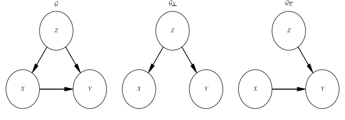
There are two causal quantities of interest \(p(Y|\mathrm{do}(X))\), the average effect, and \(p(Y|\mathrm{do}(X), Z)\), the effect on the individual. To determine them, I apply Pearl's three causal rules [1], equations (10) to (12) in the paper. To this end, I will need the modified versions of the graph shown in the schematic above. After applying causal rules, the causal effect on the individual is equal to the conditional probability in the original system
\[ \begin{aligned} P(Y|\mathrm{do}(X), Z) &= P(Y|X, Z) &&\text{per rule (II), since $(Y \perp X|Z)_{\underline{X}}$} \end{aligned} \]
Further, the distribution of \(Z\) does not change under intervention
\[ \begin{aligned} P(Z|\mathrm{do}(X)) &= P(Z) &&\text{per rule (III), since $(Z \perp X)_{\overline{X}}$} \end{aligned} \]
Combining both results, the average effect can be calculated as
\[ \begin{aligned} P(Y|\mathrm{do}(X)) &= \sum_X p(Y|\mathrm{do}(X), Z) P(Z|\mathrm{do}(X)) \\ &= \sum_X p(Y|X, Z) P(Z) \\ &= \sum_X \frac{p(Y, X, Z)}{P(X|Z)} \\ \end{aligned} \]
To summarize. When you are interested in the average causal effect \(P(Y|\mathrm{do}(X))\), you have to correct for the historic policy \(P(X|Z)\). When you are interested in the individual causal effect \(P(Y|\mathrm{do}(X), Z)\), you do not have correct for the historic policy \(P(X|Z)\) [2,5]. But you can and probably should. In particular, when using regularized models, as I argue below.
Given these quantities, there are two ways of using them, similar to reinforcement learning. First, one can use value-based approaches, where one tries to fit the conditional probability \(P(Y|X, Z)\) and use it to determine those actions that maximize some goal. Another approach is to use policy search and directly optimize a target policy \(\pi(X|Z)\) to maximize the expected value of some performance measure \(u(Y, X, Z)\). This approach is taken for bandits learned on logged data [4]. The expected utility under the new policy can be written as
\[ \begin{aligned} &\mathbb{E}\left[ u(Y, X, Z) | \mathrm{do}(X) \sim \pi(X|Z) \right] \\ &= \sum_{X, Y, Z} u(Y, X, Z) P(Y|\mathrm{do}(X) \sim \pi(X|Z), Z) P(Z|\mathrm{do}(X) \sim \pi(X|Z)) \\ &= \sum_{X, Y, Z} u(Y, X, Z) P(Y|\mathrm{do}(X) \sim \pi(X|Z), Z) P(Z|\mathrm{do}(X) \sim \pi(X|Z)) \\ &= \sum_{X, Y, Z} u(Y, X, Z) P(Y|X, Z) \pi(X, |Z) P(Z) \\ &= \sum_{X, Y, Z} P(Y, X, Z) u(Y, X, Z) \frac{\pi(X, |Z)}{P(X|Z)} \\ &= \mathbb{E} \left[ u(Y, X, Z) \frac{\pi(X, |Z)}{P(X|Z)} \right]. \end{aligned} \]
The last line allows to optimize \(\pi(A|X)\) directly from the observed data. However, it has a high variance and there are different approaches to improve its numerical properties (e.g., [4]). In the following, I will focus on the value-based approach and fit the conditional probability \(P(Y|X,Z)\) directly.
The question is now whether to reweight when fitting \(P(Y|X, Z)\) or not, i.e., whether to use
\[ \begin{aligned} &P(Y, X, Z) \frac{1}{P(X|Z)}, & &\text{or} & &P(Y, X, Z) \end{aligned} \]
as the dataset when fitting. These options are also known as inverse propensity
score method and direct method respectively. In sklearn-like code, the
difference would be between
est.fit(x_and_z, y, sample_weight=1/p_x_given_z)
# and
est.fit(x_and_z, y)
In theory, both fits should give the same answer. In the experiments and analytics discussed below, the first version becomes preferable when using regularization.
In addition to the direct method and inverse propensity score method, usually a third option is named, called doubly robust method. It is applicable, when the propensity score is estimated [6]. In the following, I assume access to the true propensity score and therefore do not discuss doubly robust estimation.
Inverse propensity scoring
The weight used in the calculation of \(P(Y|\mathrm{do}(X))\) is called inverse propensity weight ([2], [5]).
\[ w = \frac{1}{P(X|Z)}, \]
where \(P(X|Z)\) is typically obtained by a model fitted to the data set. Reweighting a dataset with the inverse propensity weight aims to remove the effect of the historic policy. That is, that each action is equally likely regardless of \(Z\). In essence it turns the data set into a randomized trial by removing the historic policy.
In addition to removing the historic policy, I will add back in a new fictitious policy \(\pi(X)\) independent of \(Z\). Adding such a policy does not change the causal properties of the system, but ensures that the resulting distribution is well normalized. Having another control lever, also allows to further tune the numerical properties of the scheme (or add stability to it in the first place). For this reason these weights are also called stabilized [5]. In this case, the weights read
\[ w = \frac{\pi(X)}{P(X|Z)}. \]
For discrete distributions a good default is to use the uniform distribution \(\pi(X) = 1/N_X\), which reproduces the usual behavior. For continuous distribution, I will use a normal distribution centered around zero that acts as a form of regularizer by penalizing large deviations.
Numerical Results
To start off, I will look into a simple version of this problem with discrete data. The data is simulated as follows
np.random.seed(42_21_13_7)
df = pd.DataFrame().assign(
    z=lambda df: np.random.binomial(n=1, p=0.3, size=100_000),
    x=lambda df: np.random.binomial(n=1, p=0.8 - 0.4 * df['z']),
    y=lambda df: np.random.binomial(n=1, p=0.5 + 0.4 * df['z'] - 0.2 * df['x'])
)
The result is the following table of observed counts N and counts N' after
inverse propensity weighting.
X | Y | Z | N | N' |
|---|---|---|---|---|
| 0 | 0 | 0 | 6958 | 17407 |
| 1 | 0 | 0 | 39315 | 24567 |
| 0 | 0 | 1 | 1842 | 1536 |
| 1 | 0 | 1 | 3512 | 4385 |
| 0 | 1 | 0 | 7051 | 17640 |
| 1 | 1 | 0 | 16773 | 10481 |
| 0 | 1 | 1 | 16087 | 13415 |
| 1 | 1 | 1 | 8462 | 10566 |
Calculating the effect via adjustment works as intended
\[ \sum_x (P(Y=1|X=1, Z) - P(Y=1|X=1, Z)) p(Z) \approx -0.200. \]
However, evaluating the conditional probabilities fails as expected with
\[ P(Y=1|X=1) - P(Y=0|X=0) \approx -0.353. \]
Evaluating the conditional effect \[P(Y=1|Z,X=1) - P(Y=1|Z,X=0)\] gives
Z | P(Y=1/X=1,Z) - P(Y=1/X=0,Z) | P'(Y=1/X=1,Z) - P'(Y=1/X=0,Z) |
|---|---|---|
| 0 | -0.204 | -0.204 |
| 1 | -0.191 | -0.191 |
As expected by the discussion above, it gives the exact effect difference bar some numerical fluctuations. Also, the result does not change when evaluating it in terms of the reweighted probability distribution. The reason is that the weight for each value of \(Z, X\) is the same and will drop out after normalizing the probability of \(Y\).
Next, I discuss two examples for continuous data. First, a fully Gaussian problem, where linear models are exact. Then, a more complicated example I took from this blog post for which I apply gradient boosting. In case of the first system, the data is generated via
def sample_continuous(size=100_000):
    pz = lambda df: scipy.stats.norm(np.zeros(size), 1)
    px = lambda df: scipy.stats.norm(+0.4 * df['z'], 1)
    py = lambda df: scipy.stats.norm(+1.0 * df['z'] - 0.1 * df['x'], 1)

    # the target distribution of the reweighted data set
    p_do_x = lambda df, target_var: scipy.stats.norm(0, target_var ** 0.5)

    return pd.DataFrame().assign(
        z=lambda df: pz(df).rvs(),
        x=lambda df: px(df).rvs(),
        y=lambda df: py(df).rvs(),
        w=lambda df: (
            p_do_x(df, 1.0).pdf(df['x'])
            / px(df).pdf(df['x'])
        ),
    )
For simplicity, I use equal variance for all distributions to make the regularization strength comparable across experiments. I will fit a linear model of the form \(\hat{y} = \beta_{yx} x + \beta_{yz} z\) with maximum likelihood and additional regularization.
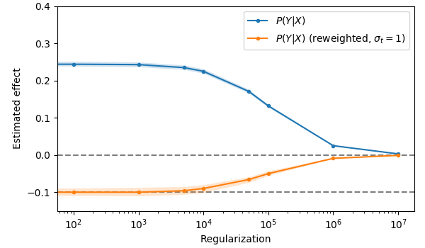
When fitting a model that does not include \(Z\), i.e., fitting \(\hat{y} = \beta_{yx} x\), the non-reweighting model (blue) is not able to fit the causal effect. The reweighted model (orange) nicely reproduces the expected effect strength of -0.1. Only at very high regularization strengths is the weight slowly shrunk to zero.
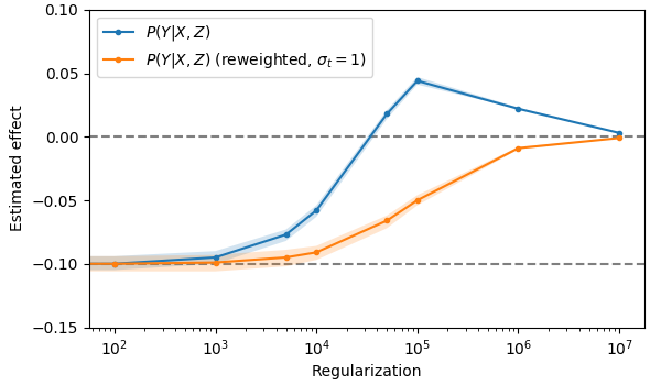
When \(Z\) is included in the model, i.e., fit \(\hat{y} = \beta_{yx} x + \beta_{yz} z\), the story becomes more complicated. At low regularization strengths both non-reweighted (blue) and reweighted (orange) models reproduce the causal effect. As the graph analysis predicted, reweighting is not required to determine the causal effect, when including \(Z\) into the model. However, as regularization strength increases, the models behave qualitatively quite different. The non regularized model starts to disagree with the true causal effect and at very high regularization strengths the estimate of the causal effect even disagrees in sign. In contrast the reweighted model always shows a consistent sign and slowly shrinks to zero as the regularization is increased. It also stays for much longer near the exact value.
Finally let's look how a more complex model behaves, say, gradient boosting. For this model, it is hard to disentangle its structural bias and regularization. For a large number of trees (100) however the model is very flexible and the learning rate acts as an regularization parameter. The example discussed so far is easily solved by gradient boosting models. Therefore, I will turn to the example used by Florian Wilhelm in his blog post. Head over to his blog post for a detailed description. In short, the dataset is a simulated drug trial and the goal is to predict
\[ \mathbb{E} \left[ \log(\text{recovery time}) | \mathrm{do}(\text{medication}), {\text{features}} \right] \]
The data set is construct such that the causal effect is exactly
\[ \begin{aligned} &\mathbb{E} \left[ \log(\text{recovery time}) | \mathrm{do}(\text{medication}), {\text{features}} \right] \\ - &\mathbb{E} \left[ \log(\text{recovery time}) | \mathrm{do}(\text{no medication}), {\text{features}} \right] \\ = &-1 \end{aligned} \]
I simulate the data as describe in Florian's blog post, but use the exact value for the probability of medication for reweighting.
def simulate(size=100_000):
    def exp_recovery_time(df):
        return df.eval(
            'exp('
            '  2 + 0.5 * sex + 0.03 * age + 2 * severity - 1 * medication'
            ')'
        )

    def rvs_recovery_time(df):
        return scipy.stats.poisson.rvs(exp_recovery_time(df))

    def get_p_medication(df):
        u = df.eval('(1 / 3 * sex + 2 / 3 * severity - 0.8) / 0.15')
        return scipy.stats.norm(0, 1).cdf(u)

    return pd.DataFrame().assign(
        sex=lambda df: np.random.randint(0, 2, size=size),
        age=lambda df: scipy.stats.gamma.rvs(8, scale=4, size=size),
        severity=lambda df: scipy.stats.beta.rvs(3, 1.5, size=size),
        medication_p=lambda df: get_p_medication(df),
        medication=lambda df: np.random.binomial(
            n=1, p=df['medication_p']
        ),
        recovery=lambda df: rvs_recovery_time(df),
        log_recovery=lambda df: df.eval('log(recovery)'),
        weight=lambda df: df.eval(
            'medication / medication_p '
            '+ (1 - medication) / (1 - medication_p)'
        ),
        no_weight=lambda df: df.eval('1'),
    )

The resulting effect estimate behaves similarly to the one in the linear model example. Initially both models estimate on average an effect close to the true effect. With increasing regularization strength (or decreasing learning rate) the error increases for both models. As with the previous example, the error increases much faster for the non-reweighted model (orange) compared to the reweighted one (blue). For typical values of the learning rate \(< 0.1\), the reweighted model always shows a better estimate for the causal effect.
To sum up: in these experiments both reweighted and non-reweighted model were able to estimate the causal effect for low regularization strengths. However, as regularization increases the effect estimates of the reweighted model match the true value much better. As I will discuss in the next sections, these effects can be derived analytically for linear regression with \(L_2\) regularization. One caveat of these simulations is, that I have used the exact propensity values, which may not be accessible in reality. In that case, predicted propensity values can be used at the cost of higher variance.
Analytical results for linear models
In the spirit of the linearization principle [3], I will focus on a fully linear system in the following discussion. For the data generating process, I assume the form
\[ \begin{aligned} z &\sim p(z) = \mathcal{N}(0, \sigma_z) \\ x &\sim p(x|z) = \mathcal{N}(\alpha_{xz} z, \sigma_x) \\ y &\sim p(y|x, z) = \mathcal{N}(\alpha_{yx} x + \alpha_{yz} z, \sigma_y) \end{aligned} \]
and fit a linear model of the form \(\hat{y} = \beta_{yx} x + \beta_{yz} z\) with \(L_2\) regularization. The resulting loss function reads
\[ \begin{aligned} \mathcal{L} &= \frac{1}{2} \langle (y - \hat{y})^2 \rangle + \frac{1}{2} \lambda \beta_{yx}^2 + \frac{1}{2} \lambda \beta_{yz}^2. \end{aligned} \]
Setting its derivatives with respect to the parameters equal to zero and solving for \(\beta_{yx}, \beta_{yz}\) gives
\[ \begin{aligned} \beta_{yx} &= \frac{ \alpha_{yx} + \frac{\lambda}{\sigma_x^2} \alpha_{xz} \left( \alpha_{yz} + \alpha_{xz} \alpha_{yx} \right) + \frac{\lambda}{\sigma_z^2} \alpha_{yx} }{ \frac{\lambda}{\sigma_x^2} \alpha_{xz}^{2} + \left(1 + \frac{\lambda}{\sigma_z^2}\right)\left(1 + \frac{\lambda}{\sigma_x^2}\right) } \\ \beta_{yz} &= \frac{ \alpha_{yz} + \frac{\lambda}{\sigma_x^2} ( \alpha_{xz} \alpha_{yx} + \alpha_{yz}) }{ \frac{\lambda}{\sigma_x^2} \alpha_{xz}^{2} + \left(1 + \frac{\lambda}{\sigma_z^2}\right)\left(1 + \frac{\lambda}{\sigma_x^2}\right) } \end{aligned} \]
When no reweighting is performed, three regimes can be distinguished.
First, a regime of weak regularization (\(\lambda \ll \sigma_x^2, \sigma_z^2\)). In this case the coefficients are close to their true values
\[ \begin{aligned} \beta_{yx} &\approx \alpha_{yx} \\ \beta_{yz} &\approx \alpha_{yz} \end{aligned} \]
In the Regime of dominant action (\(\lambda \gg \sigma_x^2, \sigma_z^2\) and \(\sigma_x^2 \gg \sigma_z^2\)), regularization is important, but variation in \(x\) is much higher than \(z\). In this case, \(z\) has hardly any influence on the prediction, and again the coefficient for \(x\) is proportional to its true value
\[ \begin{aligned} \beta_{yx} &\approx \frac{1}{1 + \lambda / \sigma_x^2} \alpha_{yx} \\ \beta_{yz} &\approx 0 \end{aligned} \]
Finally, in the regime of strong policy (\(\lambda \gg \sigma_x^2, \sigma_z^2\) and \(\sigma_z^2 \gg \sigma_x^2\)), regularization is important and the action is strongly determined by the features. Here, the policy has a strong influence. The fitted coefficients are approximately given by
\[ \begin{aligned} \beta_{yx} &\approx \frac{\alpha_{xz}^2}{1 + \alpha_{xz}^2 + \lambda / \sigma_z^2} \left( \alpha_{yz} + \alpha_{xz} \alpha_{yx} \right) \frac{1}{\alpha_{xz}} \\ \beta_{yz} &\approx \frac{1}{1 + \alpha_{xz}^2 + \lambda / \sigma_z^2} \left( \alpha_{xz} \alpha_{yx} + \alpha_{yz} \right) \end{aligned} \]
Both coefficients are proportional to the total effect of \(z\) on \(y\) and the strength of the policy \(\alpha_{xz}\) shifts the weight from one coefficient to the other. In this case, the sign of \(\beta_{yx}\) can also be opposite to \(\alpha_{yx}\).
The estimates for the coefficients change drastically when reweighting is used. Here, I will use weights \(w = \pi(X) / P(X|Z)\) with \(\pi(X) = \mathcal{N}(0, \sigma_t^2)\). This reweighting procedure has two effects on the regression coefficients. First, it effectively sets \(\alpha_{xz} = 0\). Second, it replaces the variance \(\sigma_x\) by the variance \(\sigma_t\) of the reweighting distribution. With these changes, the coefficients take the form
\[ \begin{aligned} \beta_{yx} &= \frac{\alpha_{yx}}{\left(1 + \frac{\lambda}{\sigma_t^2}\right)} \\ \beta_{yz} &= \frac{\alpha_{yz}}{\left(1 + \frac{\lambda}{\sigma_z^2}\right)} \end{aligned} \]
Now, the coefficients are always proportional to the true coefficients and only slowly go to zero as the regularization increases. In essence, the reweighting procedure has disentangled the coefficients.
Discussion
In this blog post, I investigated how causal analysis and function approximations interact. By applying Judea Pearls's causal calculus, I derived the known result that no adjustment is necessary when fitting a model conditioned on features and action [2,5]. This finding is reproduced for tabular data in numerical experiments. When applying function approximations however, the story changes. In this case, regularization makes it beneficial to perform adjustment. I demonstrated this effect numerically for linear and tree based models using simulated data and derived the effect analytically for a linear model. The disagreement between adjusted and non-adjusted models becomes more pronounced with increasing regularization strength or decreasing model capacity. This effect can be understood as a form of misspecification, which is known to cause troubles for the direct method. Only, it is not caused by the wrong functional form, but by regularization.
Consider a tree-based models: Implicitly, they will form partitions in the feature / action space. Initially, I assumed that tree-based models behave sufficiently like a tabular models for reweighting to be not necessary. However, the model averages across different partitions due to its finite capacity and thereby the model is not able to disentangle the causal effect. Even though it is hard to compare different model classes, I expect this effect to be more pronounced for random forests with their explicit averaging compared to gradient boosted trees.
As I discussed in the analytical analysis of the linear model, there are different regimes. I would argue, that the regime of strong policy is the typical one in a business setting: once a strategy has been identified, it is exploited as much as possible. It is exactly this regime, where the non-reweighted model is most likely to give wrong effect estimates (both in magnitude and sign).
So should one always reweight? In this analysis, I used the exact propensities. Already, in this case reweighting can increase variance due to finite sample effects. In real-world situations often estimated propensities are used, a procedure known to lead to high variance estimators. It is conceivable that in such a situation, it may be beneficial to vary smoothly between no reweighting and full reweighting. An example for such a weight is \(w \propto P(X|Z)^{-\nu}\) with \(\nu \ge 0\). One particular application could be vaule-based reinforcement learning in which the reweighting could be adjusted by how far back the training data was collected. Recent observations are near on-policy and would be hardly reweighted. Further back observations are more off-policy and would be subjected to stronger reweighting.
As one final thought: in essence the problems discussed in the post boil down to fitting a conditional probability distribution, when there is correlation between the variables being conditioned on. Both numerically and analytically it is beneficial to correct for these correlations. However, this is a much more general problem than predicting the influence of an action. Just consider the problem of predicting a quantity that depends both on time of year and temperature. Clearly, time of year and temperature are causally related. Following the discussion so far, I would expect the prediction to improve after correcting for this influence, at least when the temperature distribution shifts in the test data compared to the training data.
As always, I would love feedback. You can reach me on twitter via @c_prohm. In particular, if this effect is already known, I would love pointers so I can include appropriate references. The full code of all experiments and plots can be found on github here.
References
- [1]: J. Pearl "Causal diagrams for empirical research" (1995).
- [2]: J. Pearl, M. Glymour, and N. P. Jewell "Causal inference in statistics - a primer" (2016).
- [3]: Ben Recht "The Linearization Principle" http://www.argmin.net/2018/02/05/linearization/ (2018), as retrieved on Aug. 19. 2018.
- [4]: A. Swaminathan and T. Joachims "Counterfactual Risk Minimization: Learning from Logged Bandit Feedback" (2015).
- [5]: M. A. Hernán, J. M. Robins "Causal Inference", forthcoming (2018).
- [6]: M. Dudik, J. Langford, L. Li "Doubly Robust Policy Evaluation and Learning" (2011).